M9Q5-6: Molecular Orbital Theory

Chem 103 Textbook Team; Chem 104 Textbook Team

M9Q5-6: Molecular Orbital Theory

Introduction

This section explores molecular orbital (MO) theory. We will introduce molecular orbital theory and use it to describe the electronic structure of simple molecules. We will also compare and contrast the predictions of MO theory with Valence Bond theory and Lewis structures highlighting similarities and important differences. The section below provides a more detailed description of these topics, worked examples, practice problems, and a glossary of important terms.

Learning Objectives for Molecular Orbital Theory

Apply molecular orbital theory and interpret molecular orbital diagrams for simple diatomic molecules.
| Molecular Orbital (MO) Theory | MO Energy Diagrams | Bond Order | Bonding in Diatomic Molecules |

Molecular Orbital (MO) Theory

For almost every covalent molecule that exists, we can now draw the Lewis structure, predict the electron-pair geometry, predict the molecular geometry, and come close to predicting bond angles. However, one of the most important molecules we know, the oxygen molecule, O₂, presents a problem with respect to its Lewis structure. We would write the following Lewis structure for O₂:

A Lewis structure is shown. It is made up of two oxygen atoms, each with two lone pairs of electrons, bonded together with a double bond.

This electronic structure adheres to all the rules governing Lewis theory. There is an O=O double bond, and each oxygen atom has eight electrons around it. However, this picture is at odds with the magnetic behavior of oxygen. By itself, O₂ is not magnetic, but it is attracted to magnetic fields. Thus, when we pour liquid oxygen past a strong magnet, it collects between the poles of the magnet and defies gravity. Such attraction to a magnetic field is called paramagnetism, and it arises in molecules that have unpaired electrons. Experiments show that each O₂ molecule has two unpaired electrons, and yet, the Lewis structure of O₂ indicates that all electrons are paired. How do we account for this discrepancy?

Demonstration: Liquid oxygen is attracted to a magnetic field

Set up. The following demonstration shows the difference between liquid N₂ and liquid O₂ when exposed to a magnetic field.

Explanation. In this movie you can see that the N₂(ℓ) is not attracted to the horseshoe magnet and is therefore classified as diamagnetic. The O₂(ℓ), however, collects in the magnetic field until it vaporizes. This paramagnetic behavior indicates that there are unpaired electrons in O₂, yet the Lewis structure does not indicate any unpaired electrons. We need molecular orbital theory to explain this discrepancy.

Water, like most molecules, contains all paired electrons. Living things contain a large percentage of water, so they demonstrate diamagnetic behavior. If you place a frog near a sufficiently large magnet, it will levitate. You can see videos of diamagnetic floating frogs, strawberries, and more.

Molecular orbital theory (MO theory) provides an explanation of chemical bonding that accounts for the paramagnetism of the oxygen molecule. It also explains the bonding in a number of other molecules, such as violations of the octet rule and molecules with more complicated bonding (beyond the scope of this text) that are difficult to describe with Lewis structures. Additionally, it provides a model for describing the energies of electrons in a molecule and the probable location of these electrons. Unlike Valence Bond theory, which uses hybrid orbitals that are assigned to one specific atom, MO theory uses the combination of atomic orbitals to yield molecular orbitals that are delocalized over the entire molecule rather than being localized on its constituent atoms. MO theory also helps us understand why some substances are electrical conductors, others are semiconductors, and still others are insulators. Table 1 summarizes the main points of the two complementary bonding theories. Both theories provide different, useful ways of describing molecular structure.

Table 1. Comparison of Bonding Theories
Valence Bond Theory	Molecular Orbital Theory
considers bonds as localized between one pair of atoms	considers electrons delocalized throughout the entire molecule
creates bonds from overlap of atomic orbitals (s, p, d…) and hybrid orbitals (sp, sp², sp³…)	combines atomic orbitals to form molecular orbitals (σ, σ, π, π)
forms σ or π bonds	creates bonding and antibonding interactions based on which orbitals are filled
predicts molecular shape based on the number of regions of electron density	predicts the arrangement of electrons in molecules
needs multiple structures to describe resonance

Molecular orbital theory describes the distribution of electrons in molecules in much the same way that the distribution of electrons in atoms is described using atomic orbitals. Using quantum mechanics, the behavior of an electron in a molecule is still described by a wave function, Ψ, analogous to the behavior in an atom. Just like electrons around isolated atoms, electrons around atoms in molecules are limited to discrete (quantized) energies. The region of space in which a valence electron in a molecule is likely to be found is called a molecular orbital (Ψ²). Like an atomic orbital, a molecular orbital is full when it contains two electrons with opposite spin.

We will consider the molecular orbitals in molecules composed of two identical atoms (H₂ or Cl₂, for example). Such molecules are called homonuclear diatomic molecules. In these diatomic molecules, several types of molecular orbitals occur.

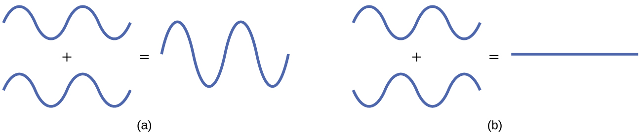
The mathematical process of combining atomic orbitals to generate molecular orbitals is called the linear combination of atomic orbitals (LCAO). The wave function describes the wavelike properties of an electron. Molecular orbitals are combinations of atomic orbital wave functions. Combining waves can lead to constructive interference, in which peaks line up with peaks, or destructive interference, in which peaks line up with troughs (Figure 1). In orbitals, the waves are three dimensional, and they combine with in-phase waves producing regions with a higher probability of electron density and out-of-phase waves producing nodes, or regions of no electron density.

A pair of diagrams are shown and labeled, “a” and “b.” Diagram a shows two identical waves with two crests and two troughs. They are drawn one above the other with a plus sign in between and an equal sign to the right. To the right of the equal sign is a much taller wave with a same number of troughs and crests. Diagram b shows two waves with two crests and two troughs, but they are mirror images of one another rotated over a horizontal axis. They are drawn one above the other with a plus sign in between and an equal sign to the right. To the right of the equal sign is a flat line. — **Figure 1.** (a) When in-phase waves combine, constructive interference produces a wave with greater amplitude. (b) When out-of-phase waves combine, destructive interference produces a wave with less (or no) amplitude.

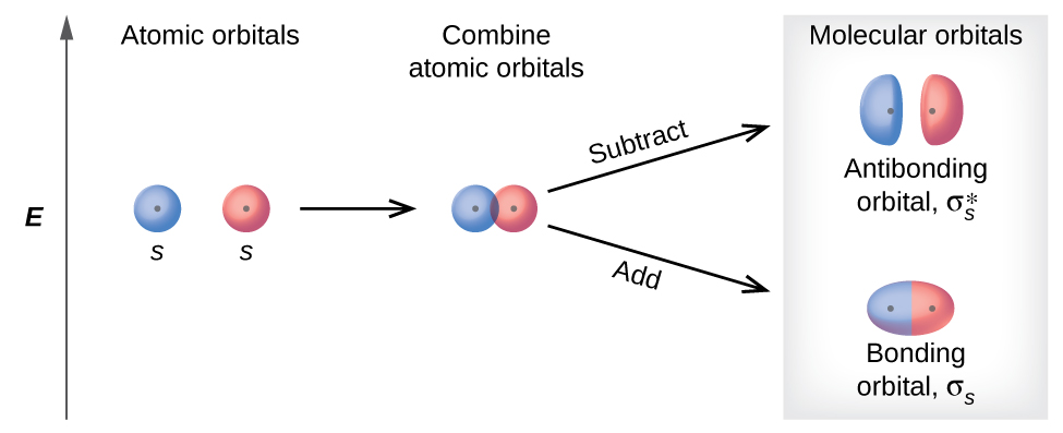
There are two types of molecular orbitals that can form from the overlap of two atomic s orbitals on adjacent atoms. The two types are illustrated in Figure 2. The in-phase combination produces a lower energy σ_s molecular orbital (read as “sigma-s”) in which most of the electron density is directly between the nuclei. The out-of-phase addition (which can also be thought of as subtracting the wave functions) produces a higher energy $\pmb \sigma^*_s$ molecular orbital (read as “sigma-s-star”) molecular orbital in which there is a node between the nuclei. The asterisk signifies that the orbital is an antibonding orbital. The σ_s orbital is of lower energy than the isolated atomic orbitals. Adding electrons to these orbitals lowers the energy of the electrons so we call these orbitals bonding orbitals. Electrons in the $\sigma^*_s$ orbitals are located in a higher energy orbital well away from the region between the two nuclei. Hence, these orbitals are called antibonding orbitals. Electrons fill the lower-energy bonding orbital before the higher-energy antibonding orbital, just as they fill lower-energy atomic orbitals before they fill higher-energy atomic orbitals.

A diagram is shown that depicts a vertical upward-facing arrow that lies to the left of all the other portions of the diagram and is labeled, “E.” To the immediate right of the midpoint of the arrow are two circles each labeled with a positive sign, the letter S, and the phrase, “Atomic orbitals.” These are followed by a right-facing horizontal arrow that points to the same two circles labeled with plus signs, but they are now touching and are labeled, “Combine atomic orbitals.” Two right-facing arrows lead to the last portion of the diagram, one facing upward and one facing downward. The upper arrow is labeled, “Subtract,” and points to two oblong ovals labeled with plus signs, and the phrase, “Antibonding orbitals sigma subscript s superscript asterisk.” The lower arrow is labeled, “Add,” and points to an elongated oval with two plus signs that is labeled, “Bonding orbital sigma subscript s.” The heading over the last section of the diagram are the words, “Molecular orbitals.” — **Figure 2.** Sigma (σ) and sigma-star (σ*) molecular orbitals are formed by the combination of two s atomic orbitals. The dots indicate the locations of nuclei.

You can watch animations visualizing the calculated atomic orbitals combining to form various molecular orbitals at the Orbitron website.

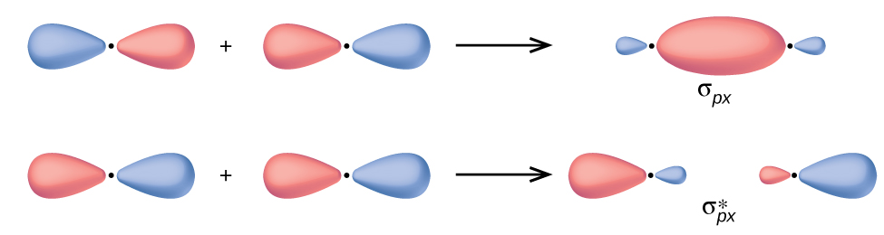
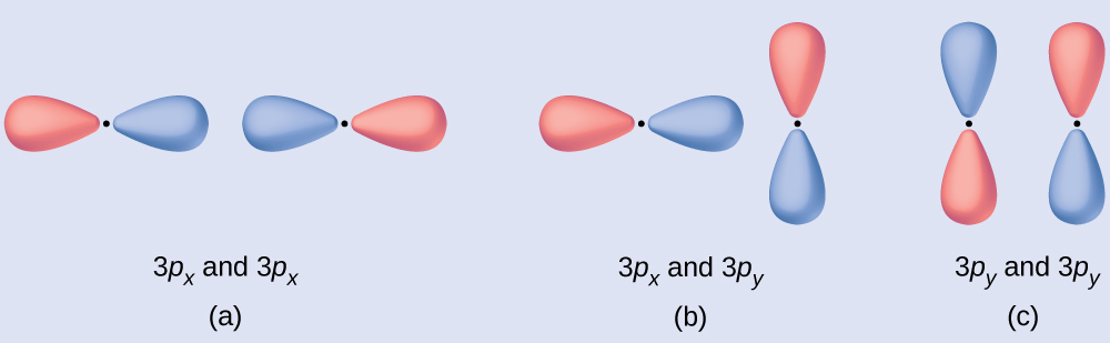
In p orbitals, the wave function gives rise to two lobes with opposite phases, analogous to how a two-dimensional wave has both parts above and below the average. We indicate the phases by shading the orbital lobes different colors. When orbital lobes of the same phase overlap, constructive wave interference increases the electron density. When regions of opposite phase overlap, the destructive wave interference decreases electron density and creates nodes. When p orbitals overlap end to end, they create σ and σ* orbitals (Figure 3). If two atoms are located along the x-axis in a Cartesian coordinate system, the two p_x orbitals overlap end to end and form σ_{p_x} (bonding) and $\sigma^*_{p_x}$ (antibonding) (read as “sigma-p-x” and “sigma-p-x star,” respectively). Just as with s-orbital overlap, the asterisk indicates the orbital with a node between the nuclei, which is a higher-energy, antibonding orbital.

Two horizontal rows of diagrams are shown. The upper diagram shows two equally-sized peanut-shaped orbitals with a plus sign in between them connected to a merged orbital diagram by a right facing arrow. The merged diagram has a much larger oval at the center and much smaller ovular orbitals on the edge. It is labeled, “sigma subscript p x.” The lower diagram shows two equally-sized peanut-shaped orbitals with a plus sign in between them connected to a split orbital diagram by a right facing arrow. The split diagram has a much larger oval at the outer ends and much smaller ovular orbitals on the inner edges. It is labeled, “sigma subscript p x superscript asterisk”. — **Figure 3.** Combining wave functions of two p atomic orbitals along the internuclear axis creates two molecular orbitals, σ_p and σ*_p.

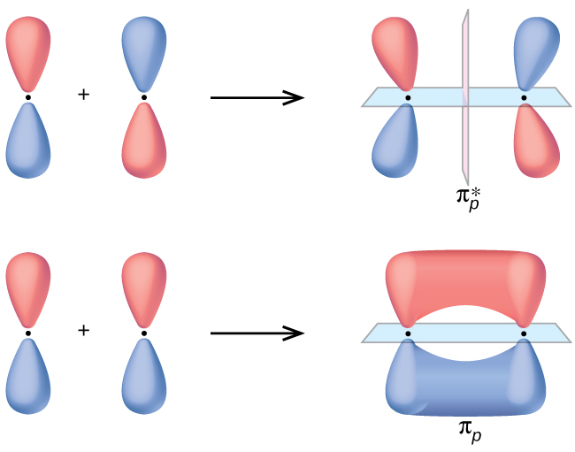
The side-by-side overlap of two p orbitals gives rise to a pi (π) bonding molecular orbital and a π* antibonding molecular orbital, as shown in Figure 4. In valence bond theory, we describe π bonds as containing a nodal plane containing the internuclear axis and perpendicular to the lobes of the p orbitals, with electron density on either side of the node. In molecular orbital theory, we describe the π orbital by this same shape, and a π bond exists when this orbital contains electrons. Electrons in this orbital interact with both nuclei and help hold the two atoms together, making it a bonding orbital. For the out-of-phase combination, there are two nodal planes created, one along the internuclear axis and a perpendicular one between the nuclei.

Two horizontal rows of diagrams are shown. The upper and lower diagrams both begin with two vertical peanut-shaped orbitals with a plus sign in between followed by a right-facing arrow. The upper diagram shows the same vertical peanut orbitals bending slightly away from one another and separated by a dotted line. It is labeled, “pi subscript p superscript asterisk.” The lower diagram shows the horizontal overlap of the two orbitals and is labeled, “pi subscript p.” — **Figure 4.** Side-by-side overlap of each two p orbitals results in the formation of two π molecular orbitals. Combining the out-of-phase orbitals results in an antibonding molecular orbital with two nodes. One contains the internuclear axis, and one is perpendicular to the axis. Combining the in-phase orbitals results in a bonding orbital. There is a node (blue) containing the internuclear axis with the two lobes of the orbital located above and below this node.

In the molecular orbitals of diatomic molecules, each atom also has two sets of p orbitals oriented side by side (p_y and p_z), so these four atomic orbitals combine pairwise to create two π orbitals and two π* orbitals. The π_{p_y} and $\pi^*_{p_y}$ orbitals are oriented at right angles to the π_{p_z} and $\pi^*_{p_z}$ orbitals. Except for their orientation, the π_{p_y} and π_{p_z} orbitals are identical and have the same energy; they are degenerate orbitals. The $\pi^*_{p_y}$ and $\pi^*_{p_x}$ antibonding orbitals are also degenerate and identical except for their orientation. A total of six molecular orbitals results from the combination of the six atomic p orbitals in two atoms: σ_{p_x} and $\sigma^*_{p_x}$ , π_{p_y} and $\pi^*_{p_y}$ , π_pz and $\pi^*_{p_z}$ .

Example 1

Molecular Orbitals
Predict what type (if any) of molecular orbital would result from adding the wave functions so each pair of orbitals shown overlap. The orbitals are all similar in energy.

Solution
(a) is an in-phase combination, resulting in a σ_3p orbital

(b) will not result in a new orbital because only orbitals with the correct alignment can combine. These orbitals do not align along the internuclear axis or in a side-by-side fashion.

(c) is an out-of-phase combination, resulting in a $\pi^*_{3p}$ orbital.

Check Your Learning
Label the molecular orbital shown as σ or π, bonding or antibonding and indicate where the node occurs.

Two orbitals are shown lying end-to-end. Each has one enlarged and one small side. The small sides are facing one another

Answer:

The orbital is located along the internuclear axis, so it is a σ orbital. There is a node bisecting the internuclear axis, so it is an antibonding orbital.

Two orbitals are shown lying end-to-end. Each has one enlarged and one small side. The small sides are facing one another and are separated by a vertical dotted line.

Walter Kohn: Nobel Laureate

Walter Kohn (Figure 5) is a theoretical physicist who studies the electronic structure of solids. His work combines the principles of quantum mechanics with advanced mathematical techniques. This technique, called density functional theory, makes it possible to compute properties of molecular orbitals, including their shape and energies. Kohn and mathematician John Pople were awarded the Nobel Prize in Chemistry in 1998 for their contributions to our understanding of electronic structure. Kohn also made significant contributions to the physics of semiconductors.

A photograph of Walter Kohn is shown. — **Figure 5.** Walter Kohn developed methods to describe molecular orbitals. (credit: image courtesy of Walter Kohn)

Kohn’s biography has been remarkable outside the realm of physical chemistry as well. He was born in Austria, and during World War II he was part of the Kindertransport program that rescued 10,000 children from the Nazi regime. His summer jobs included discovering gold deposits in Canada and helping Polaroid explain how its instant film worked.

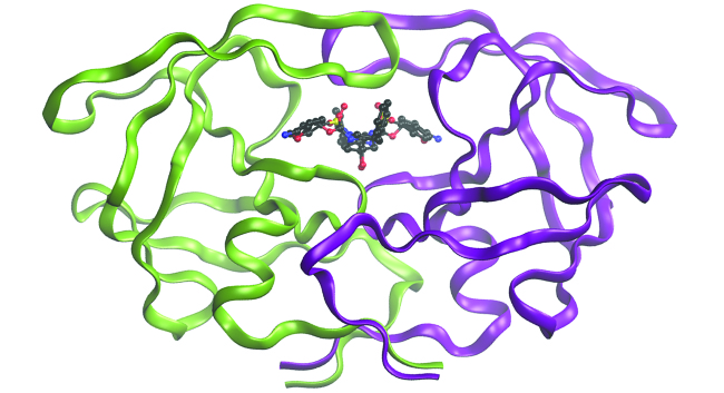
Chemistry in Real Life: Computational Chemistry in Drug Design

While the descriptions of bonding described in this module involve many theoretical concepts, they also have many practical, real-world applications. For example, drug design is an important field that uses our understanding of chemical bonding to develop pharmaceuticals. This interdisciplinary area of study uses biology (understanding diseases and how they operate) to identify specific targets, such as a binding site that is involved in a disease pathway. By modeling the structures of the binding site and potential drugs, computational chemists can predict which structures can fit together and how effectively they will bind (see Figure 6). Thousands of potential candidates can be narrowed down to a few of the most promising candidates. These candidate molecules are then carefully tested to determine side effects, how effectively they can be transported through the body, and other factors. Dozens of important new pharmaceuticals have been discovered with the aid of computational chemistry, and new research projects are underway.

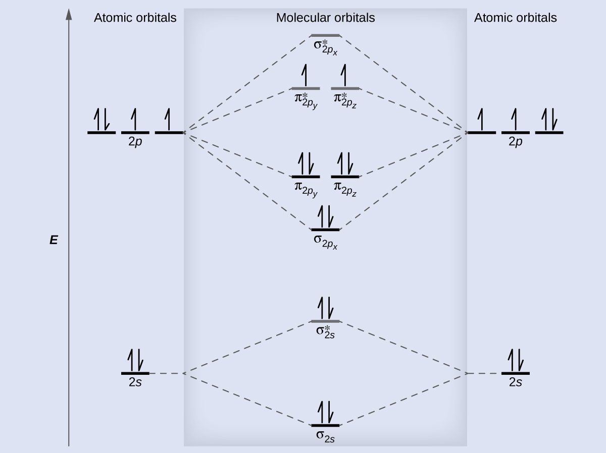
A diagram of a molecule is shown. The image shows a tangle of ribbon-like, intertwined, pink and green curling lines with a complex ball and stick model in the center. — **Figure 6.** The molecule shown, HIV-1 protease, is an important target for pharmaceutical research. By designing molecules that bind to this protein, scientists are able to drastically inhibit the progress of the disease.

Molecular Orbital Energy Diagrams

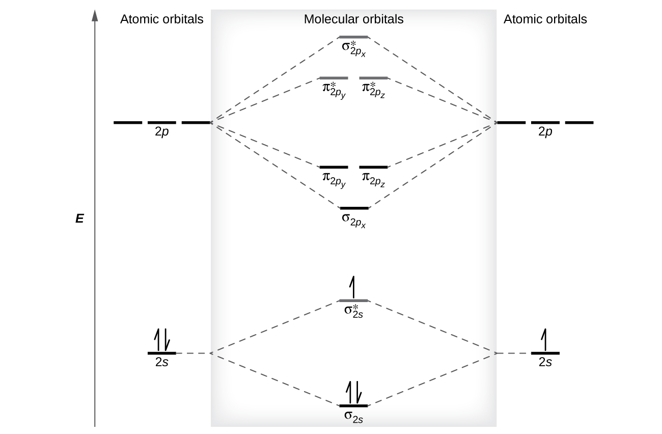
The relative energy levels of atomic and molecular orbitals are typically shown in a molecular orbital diagram (Figure 7). For a diatomic molecule, the atomic orbitals of one atom are shown on the left, and those of the other atom are shown on the right. Each horizontal line represents one orbital that can hold two electrons. The molecular orbitals formed by the combination of the atomic orbitals are shown in the center. Dashed lines show which of the atomic orbitals combine to form the molecular orbitals. For each pair of atomic orbitals that combine, one lower-energy (bonding) molecular orbital and one higher-energy (antibonding) orbital result. Thus we can see that combining the six 2p atomic orbitals results in three bonding orbitals (one σ and two π) and three antibonding orbitals (one σ* and two π*).

We predict the distribution of electrons in these molecular orbitals by filling the orbitals in the same way that we fill atomic orbitals, by the Aufbau principle. Lower-energy orbitals fill first, electrons spread out among degenerate orbitals before pairing, and each orbital can hold a maximum of two electrons with opposite spins (Figure 7). Just as we write electron configurations for atoms, we can write the molecular electronic configuration by listing the orbitals with superscripts indicating the number of electrons present. For clarity, we place parentheses around molecular orbitals with the same energy. In this case, each orbital is at a different energy, so parentheses separate each orbital. Thus we would expect a diatomic molecule or ion containing seven electrons (such as Be₂⁺) would have the molecular electron configuration $(\sigma_{1s})^2 (\sigma^*_{1s})^2 (\sigma_{2s})^2 (\sigma^*_{2s})^1$ . It is common to omit the core electrons from molecular orbital diagrams and configurations and include only the valence electrons.

A diagram is shown that has an upward-facing vertical arrow running along the left side labeled, “E.” At the bottom center of the diagram is a horizontal line labeled, “sigma subscript 2 s,” that has two vertical half arrows drawn on it, one facing up and one facing down. This line is connected to the right and left by upward-facing, dotted lines to two more horizontal lines, each labeled, “2 s.” The line on the left has two vertical half arrows drawn on it, one facing up and one facing down while the line of the right has one half arrow facing up drawn on it. These two lines are connected by upward-facing dotted lines to another line in the center of the diagram, but further up from the first. It is labeled, “sigma subscript 2 s superscript asterisk.” This horizontal line has one upward-facing vertical half-arrow drawn on it. Moving farther up the center of the diagram is a long horizontal line labeled, “sigma subscript 2 p subscript x,” which lies below two horizontal lines. These two horizontal lines lie side-by-side, and labeled, “pi subscript 2 p subscript y,” and, “pi subscript 2 p subscript z.” Both the bottom and top lines are connected to the right and left by upward-facing, dotted lines to three more horizontal lines, each labeled, “2 p.” These sets of lines are connected by upward-facing dotted lines to another single line and then pair of double lines in the center of the diagram, but farther up from the lower lines. They are labeled, “sigma subscript 2 p subscript x superscript asterisk,” and, ““pi subscript 2 p subscript y superscript asterisk,” and, “pi subscript 2 p subscript z superscript asterisk,” respectively. The left and right sides of the diagram have headers that read, ”Atomic orbitals,” while the center is header reads “Molecular orbitals”. — **Figure 7.** This is the molecular orbital diagram for the homonuclear diatomic Be₂⁺, showing the molecular orbitals of the valence shell only. On the left side are the atomic orbitals for one Be atom, and on the right are the atomic orbitals for the other Be atom. One of these Be atoms has 2 electrons in its valence shell while the other only has one (because the molecule has a +1 charge and therefore lost an electron). The molecular orbitals are filled in the same manner as atomic orbitals, using the Aufbau principle and Hund’s rule.

Bond Order

The filled molecular orbital diagram shows the number of electrons in both bonding and antibonding molecular orbitals. The net contribution of the electrons to the bond strength of a molecule is identified by determining the bond order that results from the filling of the molecular orbitals by electrons.

When using Lewis structures to describe the distribution of electrons in molecules, we define bond order as the number of bonding pairs of electrons between two atoms. Thus a single bond has a bond order of 1, a double bond has a bond order of 2, and a triple bond has a bond order of 3. We define bond order differently when we use the molecular orbital description of the distribution of electrons, but the resulting bond order is usually the same. The MO technique is more accurate and can handle cases when the Lewis structure method fails, but both methods describe the same phenomenon.

In the molecular orbital model, an electron contributes to a bonding interaction if it occupies a bonding orbital and it contributes to an antibonding interaction if it occupies an antibonding orbital. The bond order is calculated by subtracting the destabilizing (antibonding) electrons from the stabilizing (bonding) electrons. Since a bond consists of two electrons, we divide by two to get the bond order. We can determine bond order with the following equation:

bond order = $\dfrac{(\text{number of bonding electrons}) - (\text{number of antibonding electrons})}{2}$

The order of a covalent bond is a guide to its strength; a bond between two given atoms becomes stronger as the bond order increases. If the distribution of electrons in the molecular orbitals between two atoms is such that the resulting bond would have a bond order of zero, a stable bond does not form. We next look at some specific examples of MO diagrams and bond orders.

Bonding in Diatomic Molecules

A dihydrogen molecule (H₂) forms from two hydrogen atoms. When the atomic orbitals of the two atoms combine, the electrons occupy the molecular orbital of lowest energy, the σ_1s bonding orbital. A dihydrogen molecule, H₂, readily forms because the energy of a H₂ molecule is lower than that of two H atoms. The σ_1s orbital that contains both electrons is lower in energy than either of the two 1s atomic orbitals.

A molecular orbital can hold two electrons, so both electrons in the H₂ molecule are in the σ_1s bonding orbital; the electron configuration is $(\sigma_{1s})^2$ . We represent this configuration by a molecular orbital energy diagram (Figure 8) in which a single upward arrow indicates one electron in an orbital, and two (upward and downward) arrows indicate two electrons of opposite spin.

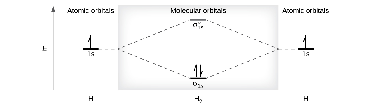
A dihydrogen molecule contains two bonding electrons and no antibonding electrons so we have

bond order in H₂= $\dfrac{(2 - 0)}{2} = 1$

Because the bond order for the H–H bond is equal to 1, the bond is a single bond.

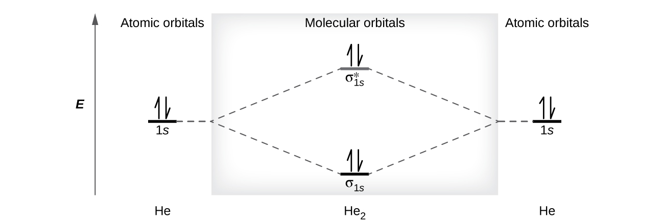
A helium atom has two electrons, both of which are in its 1s orbital. Two helium atoms do not combine to form a dihelium molecule, He₂, with four electrons, because the stabilizing effect of the two electrons in the lower-energy bonding orbital would be offset by the destabilizing effect of the two electrons in the higher-energy antibonding molecular orbital. We would write the hypothetical electron configuration of He₂ as $(\sigma_{1s})^2 (\sigma^*_{1s})^2$ as in Figure 9. The net energy change would be zero, so there is no driving force for helium atoms to form the diatomic molecule. In fact, helium exists as discrete atoms rather than as diatomic molecules. The bond order in a hypothetical dihelium molecule would be zero.

bond order in He₂= $\dfrac{(2 - 2)}{2} = 0$

A bond order of zero indicates that no bond is formed between two atoms.

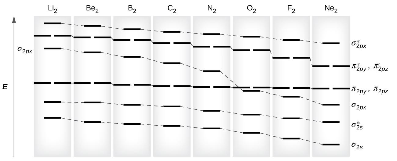
The Diatomic Molecules of the Second Period

Eight possible homonuclear diatomic molecules might be formed by the atoms of the second period of the periodic table: Li₂, Be₂, B₂, C₂, N₂, O₂, F₂, and Ne₂. However, we can predict that the Be₂ molecule and the Ne₂ molecule would not be stable. We can see this by a consideration of the molecular electron configurations (Table 2).

We predict valence molecular orbital electron configurations just as we predict electron configurations of atoms. Valence electrons are assigned to valence molecular orbitals with the lowest possible energies. Consistent with Hund’s rule, whenever there are two or more degenerate molecular orbitals, electrons fill each orbital of that type singly before any pairing of electrons takes place.

As we saw in Valence Bond theory, σ bonds are generally more stable than π bonds formed from degenerate atomic orbitals. Similarly, in molecular orbital theory, σ molecular orbitals are usually more stable than π molecular orbitals. However, this is not always the case. The MOs for the valence orbitals of the second period are shown in Figure 10. Looking at Ne₂ molecular orbitals, we see that the order is consistent with the generic diagram shown in the previous section. However, for atoms with three or fewer electrons in the p orbitals (Li through N) we observe a different pattern, in which the σ_p orbital is higher in energy than the π_p set. Obtain the molecular orbital diagram for a homonuclear diatomic ion by adding or subtracting electrons from the diagram for the neutral molecule.

A graph is shown in which the y-axis is labeled, “E,” and appears as a vertical, upward-facing arrow. Across the top, the graph reads, “L i subscript 2,” “B e subscript 2,” “B subscript 2,” “C subscript 2,” “N subscript 2,” “O subscript 2,” “F subscript 2,” and “Ne subscript 2.” Directly below each of these element terms is a single pink line, and all lines are connected to one another by a dashed line, to create an overall line that decreases in height as it moves from left to right across the graph. This line is labeled, “sigma subscript 2 p x superscript asterisk”. Directly below each of these lines is a set of two pink lines, and all lines are connected to one another by a dashed line, to create an overall line that decreases in height as it moves from left to right across the graph. It is consistently lower than the first line. This line is labeled, “pi subscript 2 p y superscript asterisk,” and, “pi subscript 2 p z superscript asterisk.” Directly below each of these double lines is a single pink line, and all lines are connected to one another by a dashed line, to create an overall line that decreases in height as it moves from left to right across the graph. It has a distinctive drop at the label, “O subscript 2.” This line is labeled, “sigma subscript 2 p x.” Directly below each of these lines is a set of two pink lines, and all lines are connected to one another by a dashed line to create an overall line that decreases very slightly in height as it moves from left to right across the graph. It is consistently lower than the third line until it reaches the point labeled, “O subscript 2.” This line is labeled, “pi subscript 2 p y,” and, “pi subscript 2 p z.” Directly below each of these lines is a single blue line, and all lines are connected to one another by a dashed line to create an overall line that decreases in height as it moves from left to right across the graph. This line is labeled, “sigma subscript 2 s superscript asterisk.” Finally, directly below each of these lines is a single blue line, and all lines are connected to one another by a dashed line to create an overall line that decreases in height as it moves from left to right across the graph. This line is labeled. “sigma subscript 2 s.” — **Figure 10.** This shows the MO diagrams for each homonuclear diatomic molecule in the second period. The orbital energies decrease across the period as the effective nuclear charge increases and atomic radius decreases. Between N₂ and O₂, the order of the orbitals changes.

You can practice labeling and filling molecular orbitals with this interactive tutorial from the University of Sydney.

This switch in orbital ordering occurs because of a phenomenon called s-p mixing. s-p mixing does not create new orbitals; it merely influences the energies of the existing molecular orbitals. The σ_s wavefunction mathematically combines with the σ_p wavefunction, with the result that the σ_s orbital becomes more stable, and the σ_p orbital becomes less stable (Figure 11). Similarly, the antibonding orbitals also undergo s-p mixing, with the σ_s^* becoming more stable and the σ_p^* becoming less stable.

A diagram is shown. At the bottom left of the diagram is a horizontal line that is connected to the right and left by upward-facing, dotted lines to two more horizontal lines. Those two lines are connected by upward-facing dotted lines to another line in the center of the diagram but farther up from the first. Each of the bottom two central lines has a vertical downward-facing arrow. Above this structure is a horizontal line that is connected to the right and left by upward-facing, dotted lines to two sets of three horizontal lines and those two lines are connected by upward-facing dotted lines to another line in the center of the diagram, but further up from the first. In between the horizontal lines of this structure are two pairs of horizontal lines that are above the first line but below the second and connected by dotted lines to the side horizontal lines. The bottom and top central lines each have an upward-facing vertical arrow. These two structures are redrawn on the right side of the diagram, but this time, the central lines of the bottom structure are moved downward in relation to the side lines. The upper portion of the structure has its central lines shifted upward in relation to the side lines. This structure also shows the bottom line appearing above the set of two lines. — **Figure 11.** Without mixing, the MO pattern occurs as expected, with the σ_p orbital lower in energy than the π_p orbitals. When s-p mixing occurs, the orbitals shift as shown, with the σ_p orbital higher in energy than the π_p orbitals.

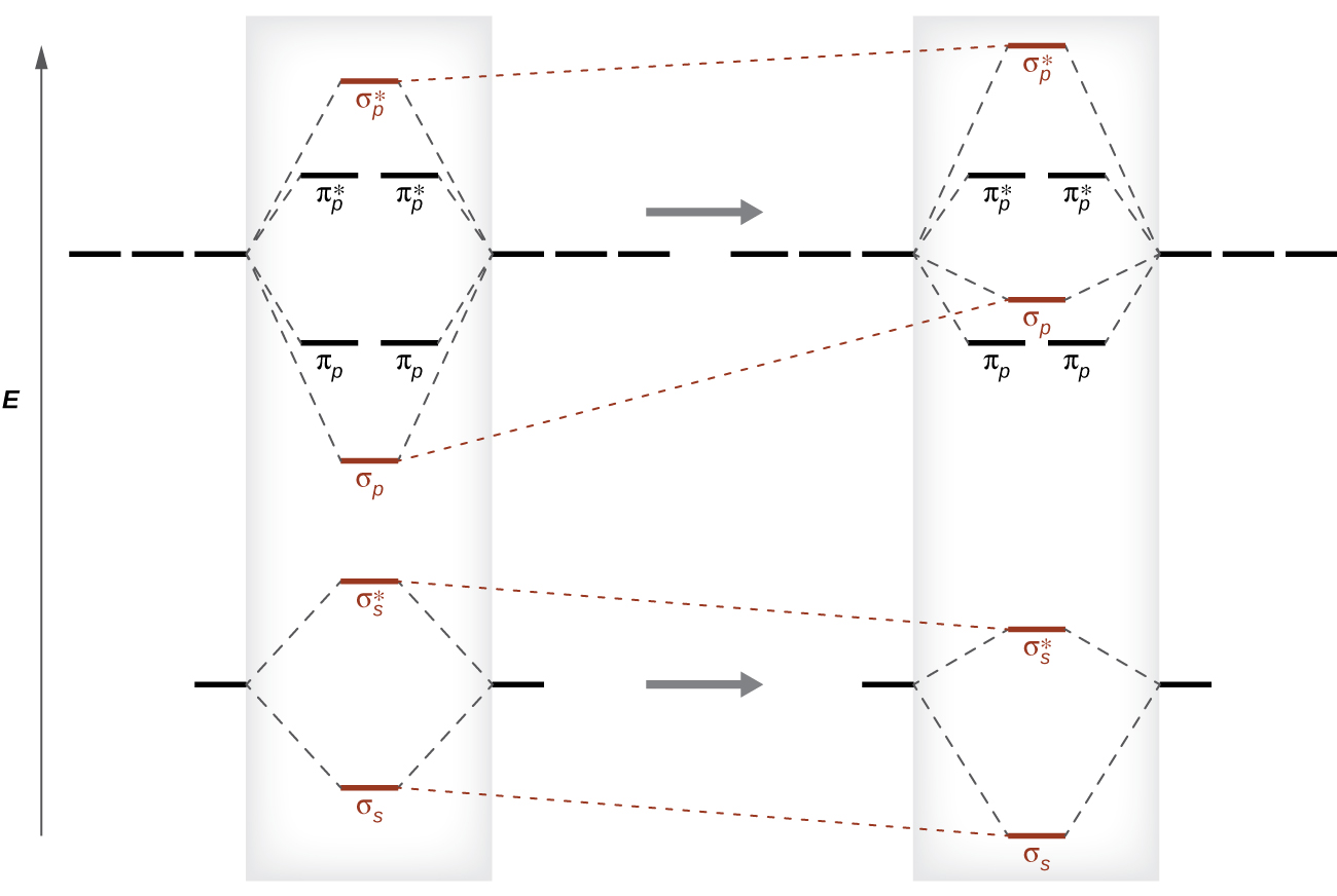
s-p mixing occurs when the s and p orbitals have similar energies. When a single p orbital contains a pair of electrons, the act of pairing the electrons raises the energy of the orbital. Thus the 2p orbitals for O, F, and Ne are higher in energy than the 2p orbitals for Li, Be, B, C, and N. Because of this, O₂, F₂, and Ne₂ only have negligible s-p mixing (not sufficient to change the energy ordering), and their MO diagrams follow the normal pattern, as shown in Figure 10. All of the other period 2 diatomic molecules do have s-p mixing, which leads to the pattern where the σ_p orbital is raised above the π_p set.

Using the MO diagrams shown in Figure 10, we can add in the electrons and determine the molecular electron configuration and bond order for each of the diatomic molecules. As shown in Table 2, Be₂ and Ne₂ molecules would have a bond order of 0, and these molecules do not exist.

Table 2. Electron Configuration and Bond Order for Molecular Orbitals in Homonuclear Diatomic Molecules of Period Two Elements
Molecule	Electron Configuration	Bond Order
Li₂	$(\sigma_{2s})^2$	1
Be₂ (unstable)	$(\sigma_{2s})^2 (\sigma^*_{2s})^2$	0
B₂	$(\sigma_{2s})^2 (\sigma^*_{2s})^2 (\pi_{2p_y}, \pi_{2p_z})^2$	1
C₂	$(\sigma_{2s})^2 (\sigma^*_{2s})^2 (\pi_{2p_y}, \pi_{2p_z})^4$	2
N₂	$(\sigma_{2s})^2 (\sigma^*_{2s})^2 (\pi_{2p_y}, \pi_{2p_z})^4 (\sigma_{2p_x})^2$	3
O₂	$(\sigma_{2s})^2 (\sigma^_{2s})^2 (\sigma_{2p_x})^2 (\pi_{2p_y}, \pi_{2p_z})^4 (\pi^_{2p_y}, \pi^*_{2p_z})^2$	2
F₂	$(\sigma_{2s})^2 (\sigma^_{2s})^2 (\sigma_{2p_x})^2 (\pi_{2p_y}, \pi_{2p_z})^4 (\pi^_{2p_y}, \pi^*_{2p_z})^4$	1
Ne₂ (unstable)	$(\sigma_{2s})^2 (\sigma^_{2s})^2 (\sigma_{2p_x})^2 (\pi_{2p_y}, \pi_{2p_z})^4 (\pi^_{2p_y}, \pi^_{2p_z})^4 (\sigma^_{2p_x})^2$	0

The combination of two lithium atoms to form a lithium molecule, Li₂, is analogous to the formation of H₂, but the atomic orbitals involved are the valence 2s orbitals. Each of the two lithium atoms has one valence electron. Hence, we have two valence electrons available for the σ_2s bonding molecular orbital. Because both valence electrons would be in a bonding orbital, we would predict the Li₂ molecule to be stable. The molecule is, in fact, present in appreciable concentration in lithium vapor at temperatures near the boiling point of the element. All of the other molecules in Table 2 with a bond order greater than zero are also known.

The O₂ molecule has enough electrons to half fill the ( $\pi^*_{2p_y}, \pi^*_{2p_z}$ ) level. We expect the two electrons that occupy these two degenerate orbitals to be unpaired, and this molecular electronic configuration for O₂ is in accord with the fact that the oxygen molecule has two unpaired electrons (Figure 12). The presence of unpaired electrons from the discussion of paramagnetism at the beginning of this section has proved to be difficult to explain using Lewis structures, but the molecular orbital theory explains it quite well. In fact, the unpaired electrons of the oxygen molecule provide a strong piece of support for the molecular orbital theory.

Example 2

Molecular Orbital Diagrams, Bond Order, and Number of Unpaired Electrons
Draw the molecular orbital diagram for the oxygen molecule, O₂. From this diagram, calculate the bond order for O₂. How does this diagram account for the paramagnetism of O₂?

Solution

We draw a molecular orbital energy diagram similar to that shown in Figure 10. Each oxygen atom contributes six electrons, so the diagram appears as shown in Figure 12.

We calculate the bond order as

O₂ = $\dfrac{8 - 4}{2}$ = 2

Oxygen’s paramagnetism is explained by the presence of two unpaired electrons in the $\pi^{*}_{2p_y}$ and $\pi^{*}_{2p_z}$ molecular orbitals.

Check Your Learning

The main component of air is N₂. From the molecular orbital diagram of N₂, predict its bond order and whether it is diamagnetic or paramagnetic.

Answer:

N₂ has a bond order of 3 and is diamagnetic.

Example 3

Ion Predictions with MO Diagrams
Give the molecular orbital configuration for the valence electrons in C₂²⁻. Will this ion be stable?

Solution

Looking at the appropriate MO diagram, we see that the π orbitals are lower in energy than the σ_p orbital. The valence electron configuration for C₂ is $(\sigma_{2s})^2 (\sigma^*_{2s})^2 (\pi_{2p_y}, \pi_{2p_z})^4$ . Adding two more electrons to generate the C₂²⁻ anion will give a valence electron configuration of $(\sigma_{2s})^2 (\sigma^*_{2s})^2 (\pi_{2p_y}, \pi_{2p_z})^4 (\sigma_{2p_x})^2$ . Since this has six more bonding electrons than antibonding, the bond order will be 3, and the ion should be stable.

Check Your Learning

How many unpaired electrons would be present on a Be₂²⁻ ion? Would it be paramagnetic or diamagnetic?

Answer:

two unpaired electrons, paramagnetic

Creating molecular orbital diagrams for molecules with more than two atoms relies on the same basic ideas as the diatomic examples presented here. However, with more atoms, computers are required to calculate how the atomic orbitals combine. See three-dimensional drawings of the molecular orbitals for C₆H₆.

Key Concepts and Summary

Molecular orbital (MO) theory describes the behavior of electrons in a molecule in terms of combinations of the atomic wave functions. The resulting molecular orbitals may extend over all the atoms in the molecule. Bonding molecular orbitals are formed by in-phase combinations of atomic wave functions, and electrons in these orbitals stabilize a molecule. Antibonding molecular orbitals result from out-of-phase combinations of atomic wave functions and electrons in these orbitals make a molecule less stable. Molecular orbitals located along an internuclear axis are called σ MOs. They can be formed from s orbitals or from p orbitals oriented in an end-to-end fashion. Molecular orbitals formed from p orbitals oriented in a side-by-side fashion have electron density on opposite sides of the internuclear axis and are called π orbitals.

We can describe the electronic structure of diatomic molecules by applying molecular orbital theory to the valence electrons of the atoms. Electrons fill molecular orbitals following the same rules that apply to filling atomic orbitals; Hund’s rule and the Aufbau principle tell us that lower-energy orbitals will fill first, electrons will spread out before they pair up, and each orbital can hold a maximum of two electrons with opposite spins. Materials with unpaired electrons are paramagnetic and attracted to a magnetic field, while those with all-paired electrons are diamagnetic and repelled by a magnetic field. Correctly predicting the magnetic properties of molecules is an advantage of molecular orbital theory over Lewis structures and Valence Bond theory.

Key Equations

bond order = $\dfrac{(\text{number of bonding electron}) - (\text{number of antibonding electrons})}{2}$

Glossary

antibonding orbital: molecular orbital located outside of the region between two nuclei; electrons in an antibonding orbital destabilize the molecule

bond order: number of pairs of electrons between two atoms; it can be found by the number of bonds in a Lewis structure or by the difference between the number of bonding and antibonding electrons divided by two

bonding orbital: molecular orbital located between two nuclei; electrons in a bonding orbital stabilize a molecule

degenerate orbitals: orbitals that have the same energy

homonuclear diatomic molecule: molecule consisting of two identical atoms

linear combination of atomic orbitals: technique for combining atomic orbitals to create molecular orbitals

molecular orbital: region of space in which an electron has a high probability of being found in a molecule

molecular orbital diagram: visual representation of the relative energy levels of molecular orbitals

molecular orbital theory: model that describes the behavior of electrons delocalized throughout a molecule in terms of the combination of atomic wave functions

π bonding orbital: molecular orbital formed by side-by-side overlap of atomic orbitals, in which the electron density is found on opposite sides of the internuclear axis

π* antibonding orbital: antibonding molecular orbital formed by out of phase side-by-side overlap of atomic orbitals, in which the electron density is found on both sides of the internuclear axis, and there is a node between the nuclei

σ bonding orbital: molecular orbital in which the electron density is found along the axis of the bond

σ* antibonding orbital: antibonding molecular orbital formed by out-of-phase overlap of atomic orbital along the axis of the bond, generating a node between the nuclei

s-p mixing: change that causes σ_p orbitals to be less stable than π_p orbitals due to the mixing of s and p-based molecular orbitals of similar energies.

Chemistry End of Section Exercises

Sketch the distribution of electron density in the bonding and antibonding molecular orbitals formed from two s orbitals and from two p orbitals.
How are the following similar, and how do they differ?
1. σ molecular orbitals and π molecular orbitals
2. bonding orbitals and antibonding orbitals
If molecular orbitals are created by combining five atomic orbitals from atom A and five atomic orbitals from atom B combine, how many molecular orbitals will result?
Can a molecule with an odd number of electrons ever be diamagnetic? Explain why or why not.
Can a molecule with an even number of electrons ever be paramagnetic? Explain why or why not.
Why are bonding molecular orbitals lower in energy than the parent atomic orbitals?
Calculate the bond order for an ion with this configuration:
$(\sigma_{2s})^2 (\sigma^*_{2s})^2 (\sigma_{2p_x})^2 (\pi_{2p_y} , \pi_{2p_z})^4 (\pi^*_{2p_y} , \pi^*_{2p_z})^3$
Determine the bond order of each member of the following groups, and determine which member of each group is predicted by the molecular orbital model to have the strongest bond.
1. H₂, H₂⁺, H₂⁻
2. O₂, O₂²⁺, O₂²⁻
3. Li₂, Be₂⁺, Be₂
4. F₂, F₂⁺, F₂⁻
5. N₂, N₂⁺, N₂⁻
For the first ionization energy for an N₂ molecule, what molecular orbital is the electron removed from?
Compare the atomic and molecular orbital diagrams to identify the member of each of the following pairs that has the higher first ionization energy (the more tightly bound electron) in the gas phase:
1. H and H₂
2. N and N₂
3. O and O₂
4. C and C₂
5. B and B₂
Which of the period 2 homonuclear diatomic molecules are predicted to be paramagnetic?
Do you agree with the following statement: The 2s orbital for fluorine starts off at a much lower energy than the 2s orbital for lithium, so the resulting σ_2s molecular orbital in F₂ is more stable than in Li₂.
True or false: Boron contains 2s²2p¹ valence electrons, so only one p orbital is needed to form molecular orbitals.
What charge would be needed on F₂ to generate an ion with a bond order of 2?
Explain why N₂²⁺ is diamagnetic, while O₂⁴⁺, which has the same number of valence electrons, is paramagnetic.
The molecular orbital filling order for diatomic nitrogen-oxygen species is: $(\sigma_{2s}) (\sigma^*_{2s}) (\sigma_{2p}) (\pi_{2p}) (\pi^*_{2p}) (\sigma^*_{2p})$ . Which of the following molecules: NO⁺, NO and NO^– is/are paramagnetic?
Consider the application of molecular orbital theory to a diatomic molecule. Which of the following statements is not correct?
1. The σ^*_2p antibonding molecular orbital is higher in energy than the σ_2p bonding molecular orbital.
2. In π molecular orbitals, electron density is centered around the internuclear axis.
3. Two atomic orbitals combine together to form two molecular orbitals.
4. A molecular orbital can hold a maximum of two electrons with the opposite spin.
5. Antibonding molecular orbitals contain a node of zero electron density between the two nuclei.

Answers to Chemistry End of Section Exercises

(a) Similarities: Both are bonding orbitals that can contain a maximum of two electrons. Differences: σ orbitals are end-to-end combinations of atomic orbitals, whereas π orbitals are formed by side-by-side overlap of orbitals.
(b) Similarities: Both are orbitals that can contain two electrons. Differences: Bonding orbitals result in holding two or more atoms together. Antibonding orbitals have the effect of destabilizing any bonding that has occurred.
Ten
An odd number of electrons can never be paired, regardless of the arrangement of the molecular orbitals. It will always be paramagnetic.
Yes, if degenerate molecular orbitals aren’t completely filled there can be an even number of unpaired electrons.
Bonding orbitals have electron density in close proximity to more than one nucleus. The interaction between the bonding positively charged nuclei and negatively charged electrons stabilizes the system.
1.5
(a) H₂ bond order = 1, H₂⁺ bond order = 0.5, H₂⁻ bond order = 0.5, strongest bond is H₂
(b) O₂ bond order = 2, O₂²⁺ bond order = 3; O₂²⁻ bond order = 1, strongest bond is O₂²⁺
(c) Li₂ bond order = 1, Be₂⁺ bond order = 0.5, Be₂ bond order = 0, strongest bond is Li₂
(d) F₂ bond order = 1, F₂⁺ bond order = 1.5, F₂⁻ bond order = 0.5, strongest bond is F₂⁺
(e) N₂ bond order = 3, N₂⁺ bond order = 2.5, N₂⁻ bond order = 2.5, strongest bond is N₂
σ_{2p_x}
(a) H₂; (b) N₂; (c) O; (d) C₂; (e) B₂
B₂ and O₂
Yes, fluorine is a smaller atom than Li, so atoms in the 2s orbital are closer to the nucleus and more stable.
False.
2+
N₂ has s-p mixing, so the π orbitals are the last filled in N₂²⁺. O₂ does not have s-p mixing, so the σ_p orbital fills before the π orbitals.
NO and NO^–
B

Comments
Please use this form to report any inconsistencies, errors, or other things you would like to change about this page. We appreciate your comments. 🙂

License

Icon for the Creative Commons Attribution-NonCommercial-ShareAlike 4.0 International License

Chem 103/104 Resource Book Copyright © by Chem 103 Textbook Team and Chem 104 Textbook Team is licensed under a Creative Commons Attribution-NonCommercial-ShareAlike 4.0 International License, except where otherwise noted.