
D3.1 Atomic Orbitals and Quantum Numbers
Quantum Numbers: n, ℓ, mℓ
The atomic wave functions can be defined using three quantum numbers: n, ℓ, and mℓ. Each wave function corresponds to an atomic orbital. Each atomic orbital defines a region in the atom within which electron probability density is large.
The energy of a hydrogen atom orbital depends on the principal quantum number, n:

As discussed earlier, the size of the orbital (the average distance of the electron from the nucleus) increases as n increases. The farther the electron is from the nucleus, the higher (less negative) the energy is.
The second quantum number, ℓ, is the orbital quantum number (sometimes called azimuth or angular-momentum quantum number). It determines the shape of the electron-density distribution. ℓ is an integer with values ranging from 0 to n – 1; that is, ℓ = 0, 1, 2, …, n – 1. Thus, an orbital with n = 1 can have only one value of ℓ, ℓ = 0, whereas n = 2 permits ℓ = 0 and ℓ = 1, and so on.
Values of ℓ are designated using letters:
| ℓ = 0 | s orbitals |
| ℓ = 1 | p orbitals |
| ℓ = 2 | d orbitals |
| ℓ = 3 | f orbitals |
| ℓ = 4 | g orbitals |
| ℓ = 5 | h orbitals |
In your class notebook write a description of the shape of the electron density distribution for each orbital shown in videos below. Also, make a rough drawing of the corresponding boundary-surface diagram for each dot-density diagram.
1s orbital
2p orbital
3d orbital
The magnetic quantum number, mℓ, specifies the spatial orientation of a particular orbital. Values of mℓ can be any integer from –ℓ to ℓ. For example, for an s orbital, ℓ = 0, and the only value of mℓ is 0; thus there is only a single s orbital. For p orbitals, ℓ = 1, and mℓ can be equal to –1, 0, or +1; thus there are three different p orbitals, which are commonly shown as px, py, and pz, oriented along the x, y, and z axes.
The total number of possible orbitals with the same value of ℓ is 2ℓ + 1. There are five d orbitals, seven f orbitals, and so forth. The sizes and shapes of s, p, and d orbitals in the first three shells are shown in the figure below. Each of these orbitals corresponds to a different set of n, ℓ, and mℓ values.
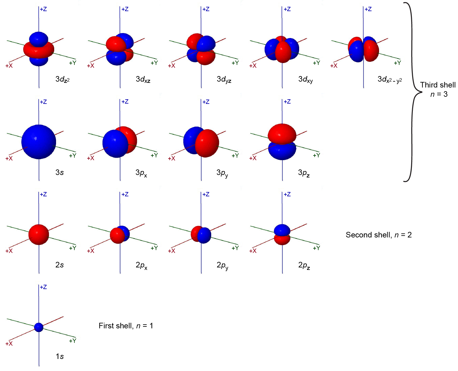
All orbitals with the same value of n and ℓ form a subshell. For example, the 2px, 2py, and 2pz orbitals constitute the 2p subshell because each of these orbitals has n = 2 and ℓ = 1. The number of orbitals in a subshell equals the number of different values for the mℓ quantum number. Each shell contains n subshells: for example, when n = 3, there is a 3s, a 3p, and a 3d subshell, corresponding to the three possible ℓ values of 0, 1 and 2.
Orbital Phases and Nodes
The figure above (Figure: Sizes and Shapes of Electron-density Distributions) shows some atomic orbitals as either all blue or all red (for example, 1s and 2s), while other orbitals contain both colors (for example, the 2p orbitals). The blue and red colors denote the mathematical sign of the wave function, a property called the phase of the wave function. Most wave functions are positive in some regions and negative in others. Phase is important when wave functions on two atoms interact to form a chemical bond.
The relationship between wave function and electron density is depicted more explicitly in the figure below. In the middle row, boundary-surface diagrams show the sizes and shapes of electron-density distributions for the 1s, 2s, and one of the 2p orbitals. In the top row are the corresponding wave functions (ψ); the bottom row shows electron density, ψ2.
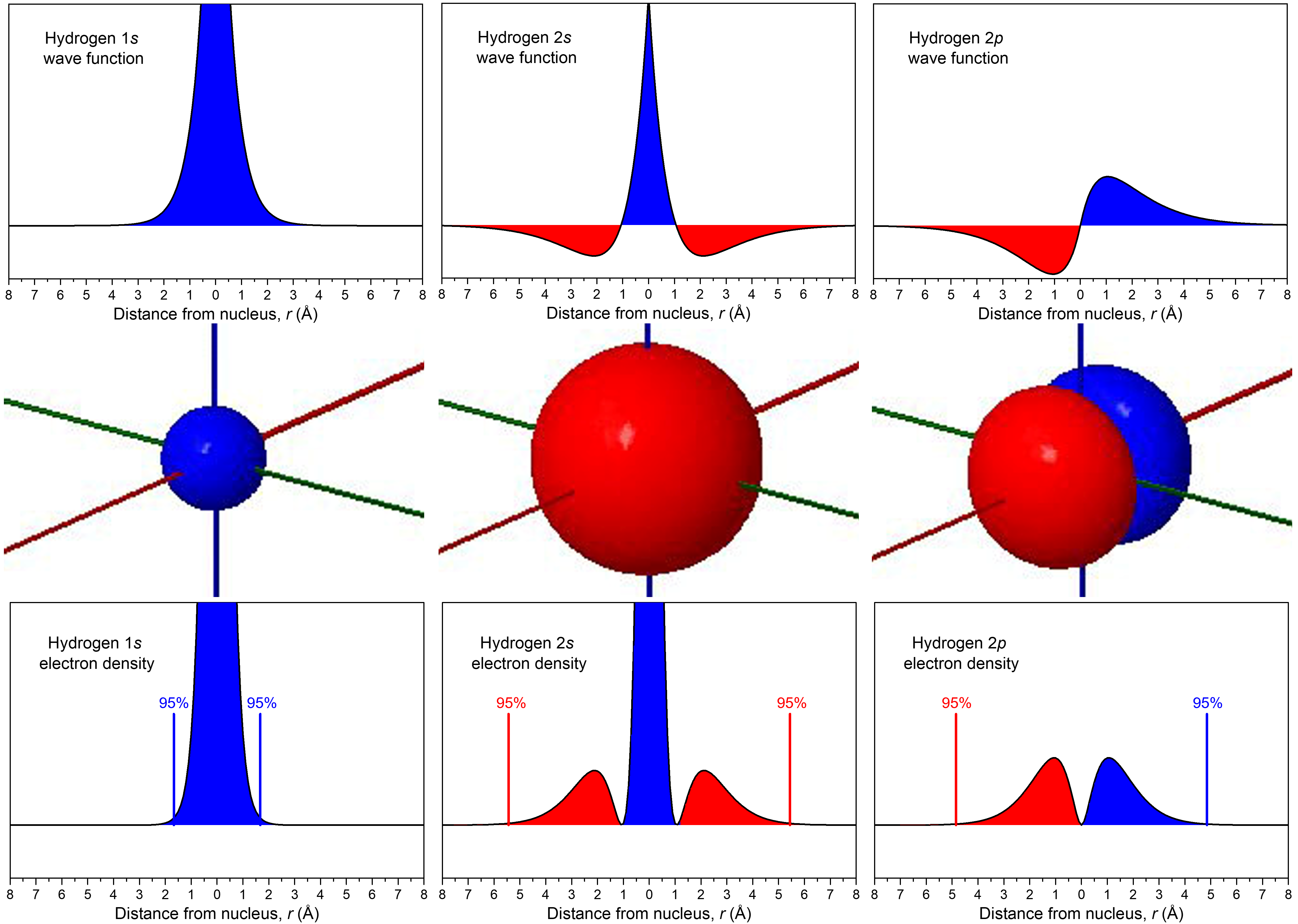
The wave functions and electron-density functions are color coded to show the regions where ψ > 0 as blue and the areas where ψ < 0 as red. A surface where the wave function changes sign is called a node. At a node, ψ = 0 and therefore the probability of finding the electron in that surface is also 0.
For the 1s orbital, there are no nodes; its wave function only has positive values. For the 2s orbital, there is one node at r = 1.05 Å; the wave function goes from positive values near the nucleus to negative values farther out. (You cannot see this node in the boundary-surface diagram, because the node is a sphere that is within the volume enclosed by the boundary surface.) A node that occurs at a specific value of r is a radial node, and therefore radial nodes have a spherical shape. The 3s orbital, for example, has two radial nodes enclosed within the boundary-surface diagram.
Each 2p orbital has one node. Look at the boundary-surface diagram to verify that this node is planar instead of spherical. Non-spherical nodes are angular nodes. For example, the 2px orbital has one angular node: the yz plane; ψ is equal to 0 at all points in the yz plane rather than at any specific r value. You can see the presence of angular nodes clearly in boundary-surface diagrams.
An orbital has n – 1 nodes, of these, n – 1 – ℓ are radial nodes, and the number of angular nodes corresponds to the value of ℓ. A generalization that is true for all kinds of waves is that the greater the total number of nodes, the higher the energy. The phase of the wave function differs on either side of a node because the wave function changes from one mathematical sign to the other as it crosses a node. Visually, we represent these different phases, and the presence of nodes, with different colors in the boundary-surface diagram.
Fourth Quantum Number, ms
The fourth quantum number, called the spin quantum number, ms, differs from the other three quantum numbers in that it describes the electron rather than the orbital. An electron has a very small magnetic field. Moving a macroscopic charge in a circular path produces a magnetic field, so initially the electron’s magnetic field was attributed to it spinning like a top; hence the name “spin quantum number”. The electron’s magnetic field can have two quantized states: either “up” or “down”. This gives two possible ms values, ms = +½ or ms = -½. When an electron occupies an orbital, we typically depict these two possible ms values as an ↑ or ↓ arrow.
In your class notebook make a table summarizing the names, symbols, allowed values, and important properties of the four quantum numbers. (You can use this table for studying later.) If you are studying with someone else, make your tables independently and then compare.
When you are satisfied with your table, compare it with ours.
Please use this form to report any inconsistencies, errors, or other things you would like to change about this page. We appreciate your comments. 🙂
