
In Depth: The Heisenberg Uncertainty Principle
The Heisenberg Uncertainty Principle
The inability to locate an electron precisely seems strange, but it is true of all atomic-scale particles. In 1927, Werner Heisenberg introduced the Heisenberg uncertainty principle: it is fundamentally impossible to determine simultaneously and exactly both the momentum and the position of a particle. Mathematically, the Heisenberg uncertainty principle states that:

where Δx is the uncertainty in the position and Δpx is the uncertainty in the momentum along the x direction. Hence, the more accurately we measure the momentum of a particle, the less accurately we can determine its position at that time, and vice versa.
Activity 1: Uncertainty Principle
The result of your calculation shows that if an electron has Δx = 1 pm, the uncertainty in its velocity is at least 5 × 10⁷ m/s. In other words, we essentially have no idea how fast it’s moving.
Heisenberg’s principle imposes ultimate limits on what is measurable in science. It is possible to talk about the probability that the electron is at a specific location, or the probability that it is moving at a given speed, but there will also be some probability of finding it somewhere else in the box or moving at some other speed.
The uncertainty principle may seem strange, but we can say that the probability of finding a particle-like electron at a given location depends on the shape of the wave associated with the electron. Various wave shapes can be described mathematically using functions such as sines or cosines; that is, there is a mathematical wave function that describes each wave. The wave function is usually represented by a Greek letter ψ.
Shortly after the uncertainty principle was proposed, the German physicist Max Born (1882 to 1969) suggested that the square of the magnitude of the wave function, ψ2, at any position is proportional to the probability of finding the electron (as a particle) at that position. If we can determine the wave function associated with an electron, we can also determine the relative probability of the electron being located at one point as opposed to another. Thus, each wave form you drew in a previous Activity can be represented by a different function, ψn, each has a different distribution of electric charge throughout the box, and each is associated with a different, specific energy value.
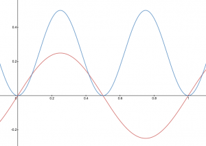
A graphic way of indicating the probability of finding the electron at a particular location is by the density of shading or stippling; that is, where the probability is high we draw lots of dots or darker shading and where the probability is low we draw fewer dots. We say that where the probability is high we have a large electron probability density (or just electron density). (In the vibrating string analogy we would draw lots of dots at places where the string was vibrating quite far from its rest position. For example, consider the wave shown below in red along with its square shown in blue. Wherever there is a maximum in the square of the wave function, we would plot a lot of dots.)
In your course notebook, annotate each of your drawings of the vibrating string with dots such that the density of dots indicates the electron probability density.
In Bohr’s theory an electron had a well-defined orbit around the nucleus, but according to the uncertainty principle, the best we can do is indicate electron density in various regions. Consequently we use a slightly different word to refer to the wave function and its electron-density distribution: orbital. The electron density of orbitals of an atom or molecule is very useful because it indicates where there is negative charge (electron density) relative to positive charge (atomic nuclei). This helps us understand atomic properties, chemical bonds, and forces between molecules.
Please use this form to report any inconsistencies, errors, or other things you would like to change about this page. We appreciate your comments. 🙂
